
How cable fault location works
A buried cable fails somewhere under a street. Finding it takes four measurements, each one narrowing the search: from the whole cable, to a distance in metres, to the spot where you dig.
Everything on this page is high-voltage work. Isolate, earth and test under your utility’s switching and safety rules before connecting any instrument.
What a cable fault is
A point where the insulation between the conductor and the earthed screen has failed, or where the conductor itself is broken. Its resistance decides how you find it.
In each sketch the top line is the conductor and the bottom line is the earthed metallic screen.
-
Open circuit
The conductor is broken. The pulse reflects back with the same polarity it was sent with.
Low-voltage TDR alone: visible
-
Short circuit
A low-resistance path from the conductor to the screen or another phase. The reflection comes back inverted.
Low-voltage TDR alone: visible
-
High-resistance
A leakage path of hundreds of ohms or more. It barely changes the cable’s impedance, so a low-voltage pulse passes it by.
Low-voltage TDR alone: hidden, condition first
-
Intermittent
Holds at low voltage and flashes over only above a certain voltage, often only in service. Between flashovers it looks healthy.
Low-voltage TDR alone: hidden, condition first
Rule of thumb: power cables have a characteristic impedance of roughly 10 to 50 Ω. A shunt fault well below that reflects strongly. One many times higher, from about a kilohm upwards, reflects too little to see, which is why many faults in medium-voltage cables need step 2 before they can be measured.
Inside a medium-voltage cable
A test pulse does not run along the copper alone. It travels between the conductor and the metallic screen, guided through the insulation. So the insulation sets its speed, and every measurement starts with knowing the cable.
- Conductor
- Stranded copper or aluminium. Carries the load current and the test pulse.
- Conductor screen
- Semiconductive layer that smooths the electric field at the strands.
- XLPE insulation
- Holds the voltage. Its permittivity sets how fast the pulse travels.
- Insulation screen
- Semiconductive layer that keeps the field inside the insulation.
- Metallic screen
- Copper wires or tape, earthed. The return path for fault current and for the pulse.
- Outer sheath
- PE or PVC, often red. Keeps water out. A damaged sheath is a fault of its own.
Velocity of propagation. In XLPE cables the pulse travels at about 160 m/µs, a little over half the speed of light. Reflectometers use half that figure, v/2, because the pulse goes out and back.
A typical v/2 for XLPE is 80 m/µs; paper-insulated cables are usually a little slower. Confirm the value on a healthy phase or a known length before you trust a distance.
Four steps, one sequence
Each step hands a narrower search to the next. Skip one and the next is guessing.
-
Step 1: Pre-locate: measure the distance
A time domain reflectometer (TDR) sends a short low-voltage pulse into the faulty phase and records what comes back. Wherever the cable’s impedance changes, part of the pulse reflects: at joints, at the cable end, and at the fault.
The time to the start of the reflection, multiplied by v/2, is the distance. An open circuit reflects with the same polarity as the pulse; a short circuit reflects inverted. The further the fault, the smaller and wider its reflection, because the cable attenuates and spreads the pulse.
- Reflection after
- 16.0µs
- v/2, XLPE, typical
- 80m/µs
- Distance to fault
- 1,280m
80 m/µs × 16.0 µs = 1,280 m to an open circuit.
Move the fault along a 2,000 m XLPE cable. Top: the cable, with the pulse going out (solid) and coming back (dashed). Below: the trace the TDR draws. The time axis and the distance axis are the same axis, scaled by v/2. - What you measure
- Round-trip time to the reflection, converted to metres with the cable’s v/2.
- Typical pitfall
- A wrong v/2. Five per cent off in velocity is five per cent off in distance: 64 m on a 1,280 m fault.
-
Step 2: Condition: make the fault visible
High-resistance and intermittent faults do not show on a low-voltage trace. A surge generator charges a capacitor to several kilovolts and discharges it into the cable. At the fault the voltage breaks down the weak insulation and an arc forms. While it burns, the arc is close to a short circuit, so for a few milliseconds the fault reflects.
With the arc reflection method (ARM), a filter couples the TDR to the cable and keeps the high voltage away from it. The TDR records one trace before the surge and one during the arc. Where the two traces part is the fault. When the arc is too short to catch, or on long cables, the impulse current method (ICM) reads the current transients of the discharge instead.
The reference shows only the cable end: the high-resistance fault is invisible to it. During the arc the fault behaves like a short and reflects inverted. - What you measure
- The distance at which the arc trace departs from the reference trace.
- Typical pitfall
- Surging higher than the fault needs. Raise the voltage in steps, and stay within the test voltage allowed for the cable.
-
Step 3: Pinpoint: find the spot to dig
A pre-located distance still carries the uncertainty of v/2 and of the route, often several metres. Digging needs the exact spot.
With the surge generator firing at a steady rate, every discharge makes a sharp thump at the fault, and the sound travels up through the soil. Walk the traced route around the pre-located distance with a ground microphone. The thump is loudest directly above the fault and fades on either side.
Compare loudness, not just presence: on hard surfaces and along ducts the sound can carry several metres.
Bar heights follow 1/r for a fault 1 m deep, ignoring soil damping: a metre off the spot the thump is already about 30% quieter. - What you measure
- The loudness of each discharge at stops along the route. The maximum marks the fault.
- Typical pitfall
- Listening while walking. Footsteps and traffic mask the thump: stand still for each shot.
-
Step 4: Trace route: put the distance on the map
The TDR measures along the cable, not across the street. A cable that turns a corner can be 1,280 m away along its length and well under 1,000 m away in a straight line. Without the route, the pinpointer walks the wrong line.
A transmitter puts an audio-frequency signal on the cable. A hand-held receiver picks up the magnetic field above it and follows the cable along the street, corner by corner. Pace the distance along the traced path, and allow for slack at joints and terminations.
In practice you trace before you walk with the pinpointer. It comes last here because it turns a distance into an address.
Same fault, two distances. Only the one along the traced route leads to the spot the pinpointer is listening for. - What you measure
- The cable’s path at the surface, and on most receivers its depth.
- Typical pitfall
- Pacing the distance in a straight line, or along the kerb instead of above the cable.
- Instruments
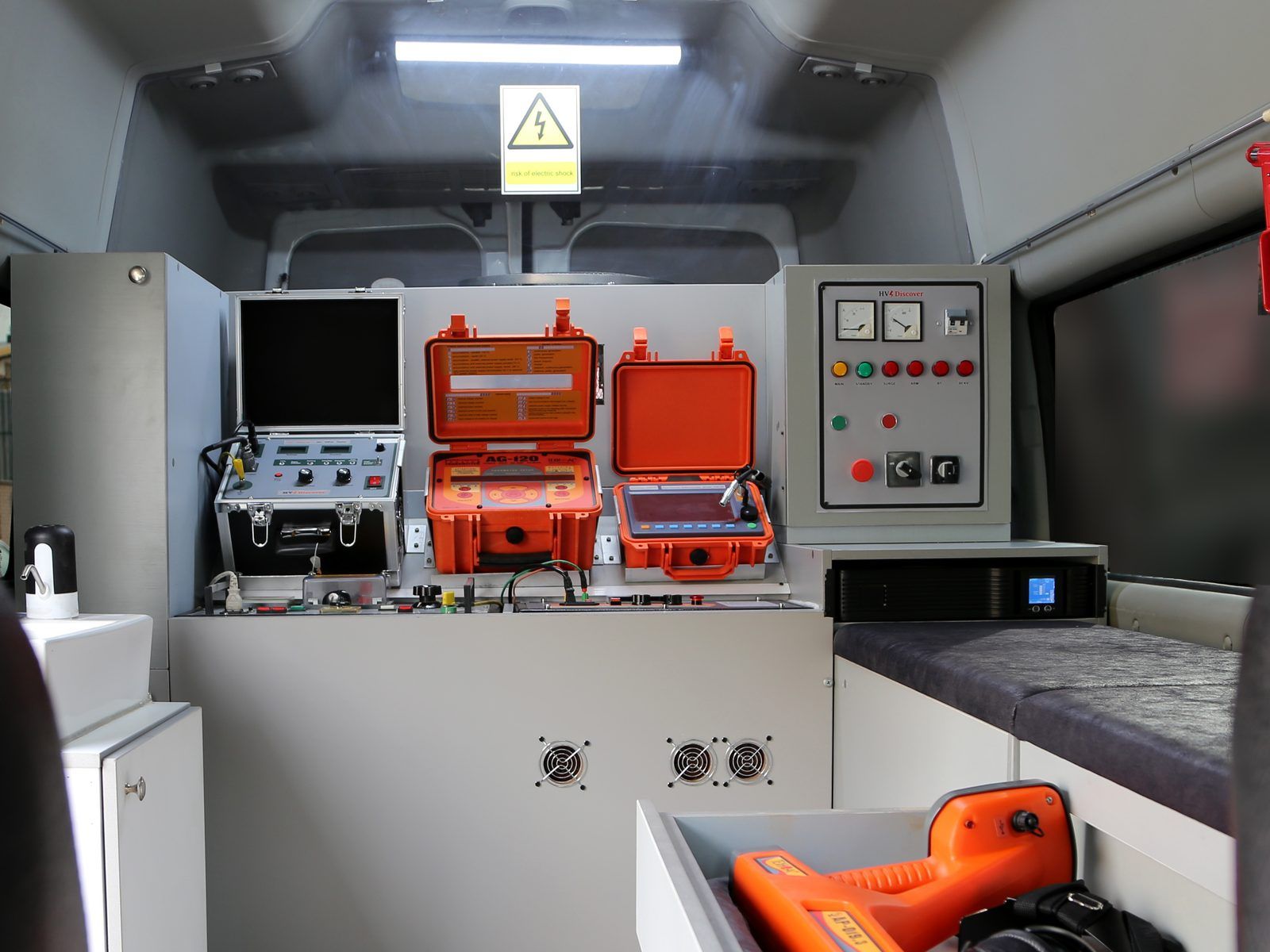
Put the whole chain in one vehicle.
The cable test van carries every step, fitted and wired: a reflectometer, a surge generator, an acoustic receiver and a route tracer, with the high-voltage connections at the rear doors. The crew arrives ready to measure.
Price the chain for your network.
Tell us the cable voltage and length, and the faults you see most. We recommend the kit and quote it.