Hospital Bed Allocation — a Discrete-Event Simulation Study

01Abstract

A small hospital ward is modelled as a discrete-event system: patients arrive at random, go through triage, and compete for a limited number of inpatient beds. When every bed is taken they wait in a bounded queue; when even the queue is full, or they wait longer than their clinically safe limit, they are turned away. The simulation is used as a decision-support tool: four ward configurations are compared over 35 independent replications each, under common random numbers, with 95% confidence intervals on every metric. The study asks three practical questions — what a modest capacity investment buys, whether a smarter queue discipline can protect urgent patients for free, and how fragile the ward is to demand variability when average demand stays exactly the same.

Rejection rate, base ward

8.6%

10 beds, queue of 5, FIFO

Rejection with +1 bed, +2 queue slots

3.6%

▼ more than halved vs base

High-priority rejection, aging queue

16.9%

▼ from 23.5% — at zero capacity cost

Rejection under Poisson arrivals

16.3%

▲ nearly ×2, at identical mean demand

02The four ward configurations

The base case is fixed by the course handout; the three alternatives are self-designed experiments, each isolating one decision a ward manager could actually make.

base

10 beds · queue 5 · FIFO · arrivals U(1, 3) h · 720 h horizon

The reference configuration, exactly as specified in the handout.

capacity_flex

11 beds · queue 7 · FIFO · arrivals U(1, 3) h

A modest, mixed capacity investment — one marginal bed plus two waiting slots, the kind of change that is actually fundable.

aging_priority

10 beds · queue 5 · aging priority queue · arrivals U(1, 3) h

Same physical capacity, but a freed bed goes to the queued patient with the highest effective score = priority + 0.6 × hours waited — urgency protection without starvation.

poisson_demand

10 beds · queue 5 · FIFO · arrivals Exp(mean 2) h

Identical average load, but memoryless and bursty — isolating the cost of variability itself.

03Results

Every cell is a mean over 35 replications with its Student-t 95% confidence interval; the same 35-seed list is reused across scenarios (common random numbers), so differences are not driven by different luck.

Bold marks the best value in each row. Full precision in `results/tables/scenario_ci_summary.csv` in the repository.
Metric (mean)	base	capacity_flex	aging_priority	poisson_demand
Admission rate	0.912[0.907, 0.918]	0.963[0.959, 0.967]	0.910[0.904, 0.915]	0.835[0.824, 0.846]
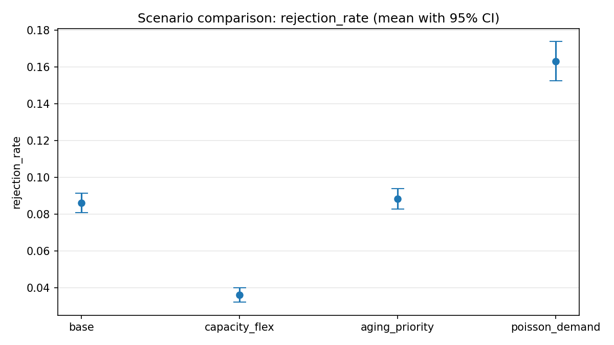
Rejection rate	0.086[0.081, 0.091]	0.036[0.032, 0.040]	0.088[0.083, 0.094]	0.163[0.152, 0.174]
Rejection, high priority	0.235[0.222, 0.248]	0.116[0.104, 0.128]	0.169[0.157, 0.182]	0.307[0.285, 0.329]
Rejection, medium priority	0.062[0.056, 0.068]	0.020[0.016, 0.023]	0.074[0.066, 0.081]	0.157[0.145, 0.169]
Rejection, low priority	0.008[0.005, 0.011]	0.002[0.000, 0.003]	0.050[0.042, 0.059]	0.052[0.043, 0.060]
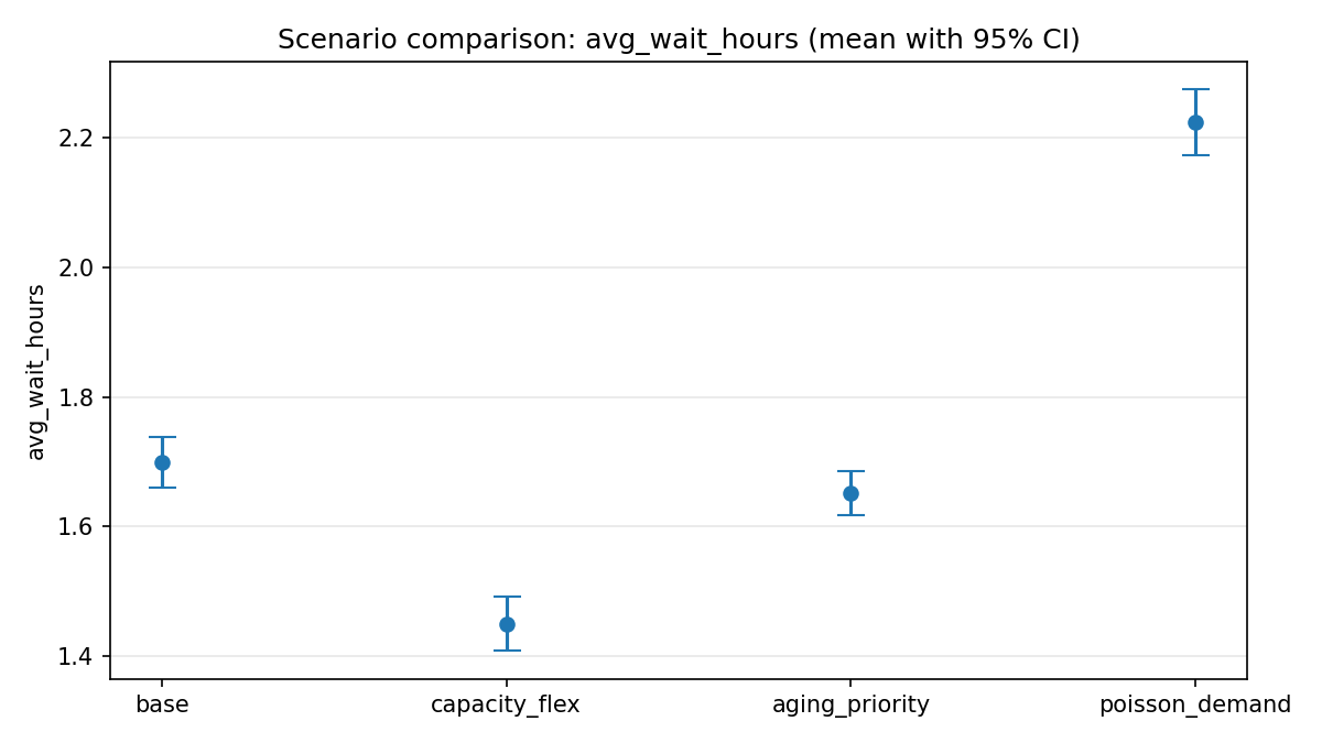
Avg queue wait (h)	1.70[1.66, 1.74]	1.45[1.41, 1.49]	1.65[1.62, 1.69]	2.22[2.17, 2.27]
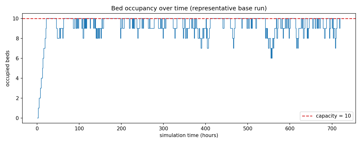
Bed utilisation	0.945[0.942, 0.948]	0.911[0.907, 0.915]	0.946[0.944, 0.949]	0.867[0.858, 0.875]
% time under pressure	38.1[36.4, 39.7]	20.9[19.4, 22.3]	40.3[38.9, 41.8]	33.0[31.2, 34.8]
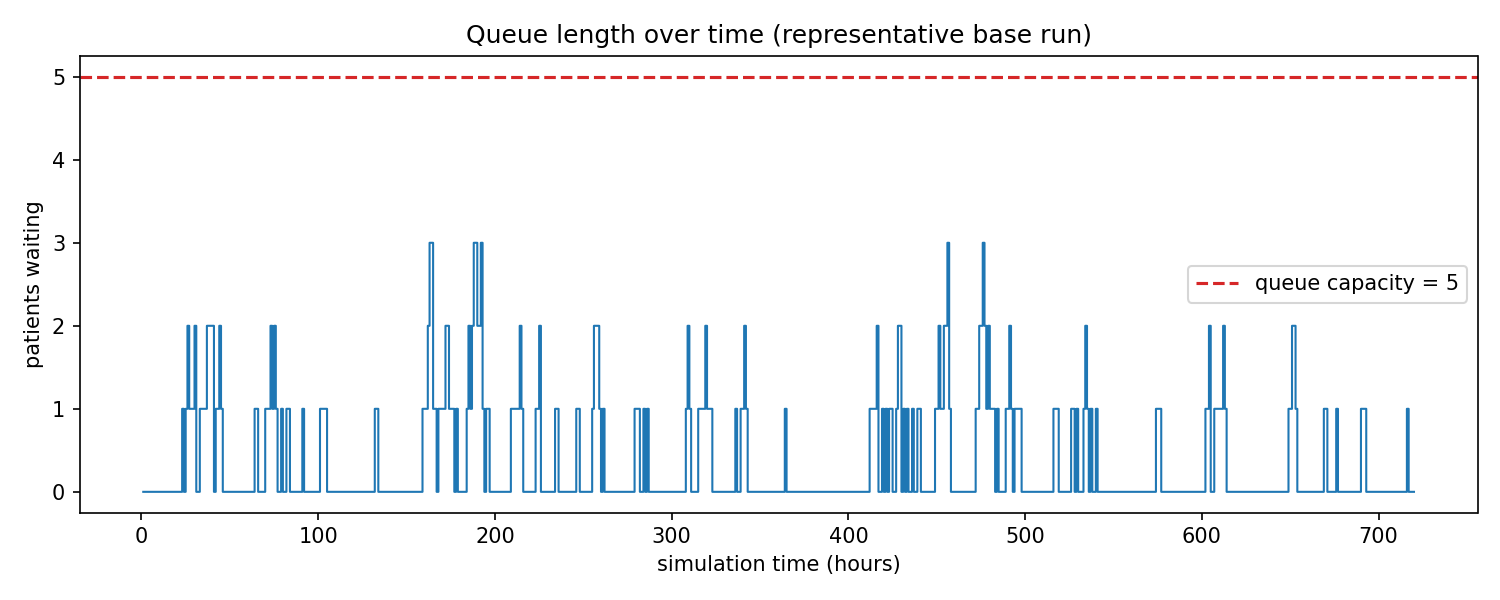
% time queue full	0.00	0.00	0.00[−0.00, 0.01]	1.00[0.82, 1.18]
Avg length of stay (h)	22.24[22.14, 22.35]	21.93[21.83, 22.04]	22.35[22.24, 22.45]	22.21[22.12, 22.31]

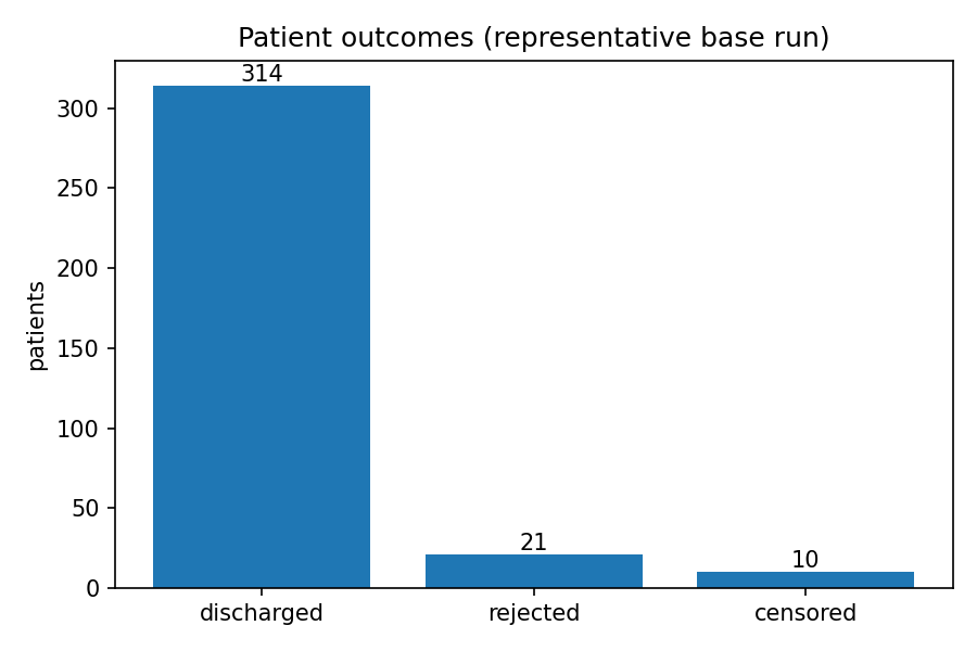
Arrivals stop at hour 720 and the clock stops hard there; patients still inside are marked censored (≈ 10 of ≈ 359 per base replication, ≈ 3%), so duration metrics use only durations completed inside the horizon.

04What the confidence intervals say

Capacity wins on every axis.
One bed plus two queue slots cuts the rejection rate by more than half — CI [0.032, 0.040] vs [0.081, 0.091], no overlap — and time under pressure from 38% to 21%, roughly 18 patients saved per month. Utilisation dips only ≈ 3 points, so the eleventh bed is genuinely used, not idle.
The aging queue is a targeted, not a global, improvement.
Overall rejection is statistically indistinguishable from base (0.088 vs 0.086, overlapping CIs) — a queue discipline cannot create capacity. What it does is redistribute: high-priority rejection falls from 23.5% to 16.9% while low-priority rejection rises from 0.8% to 5.0%, both with non-overlapping CIs. Whether that trade is good is a clinical-ethics judgement — which is exactly why it is worth simulating rather than guessing.
Variability alone is expensive.
With the same mean demand, Poisson arrivals nearly double the rejection rate (8.6% → 16.3%) yet lower utilisation (0.87 vs 0.95): bursts overwhelm the ward while lulls leave beds idle. Capacity planning against average demand alone is therefore misleading.

05Figures

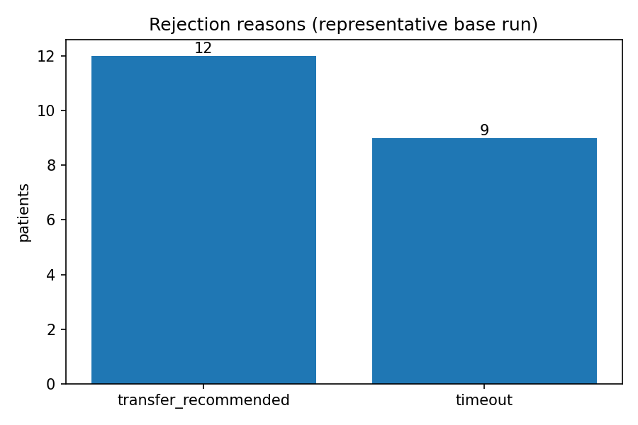
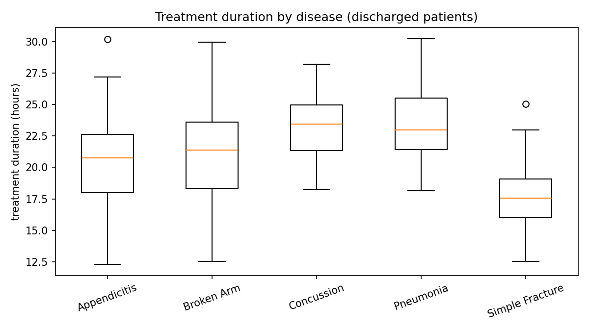
All figures regenerate bit-for-bit with python -m wardsim all; the single-run panels use a representative base replication.

Dot-and-interval chart comparing mean rejection rate with 95% confidence intervals across the four scenarios: base about 0.086, capacity_flex about 0.036, aging_priority about 0.088, poisson_demand about 0.163. — Rejection rate by scenario (mean ± 95% CI). The capacity experiment separates cleanly; the aging queue does not move the total.

Dot-and-interval chart comparing average queue wait in hours across scenarios: base about 1.70, capacity_flex about 1.45, aging_priority about 1.65, poisson_demand about 2.22. — Average queue wait by scenario (mean ± 95% CI). Poisson arrivals add half an hour at identical mean load.

Step chart of occupied beds over 720 simulated hours in a representative base run, hovering at or near the capacity line of 10 for most of the horizon. — Bed occupancy over time, representative base run — the ward sits at or near its 10-bed capacity for most of the month.

Step chart of waiting-queue length over 720 simulated hours in a representative base run, fluctuating between 0 and the queue capacity of 5. — Queue length over time, representative base run.

Bar chart of patient outcomes in a representative base run: 314 discharged, 21 rejected, 10 censored at the end of the horizon. — Patient outcomes, representative base run: 314 discharged, 21 rejected, 10 censored by the horizon.

Bar chart of rejection and early-departure reasons in a representative base run, split by queue-full rejections and tolerance expiries. — Why patients are lost: queue-full rejections vs wait-tolerance expiries (transfer recommended / timeout / non-urgent).

Chart of treatment durations grouped by disease, showing each disease's uniform base range widened upward by severity. — Treatment duration by disease — the Appendix-A range per disease, stretched upward by per-patient severity.

06Method, in brief

Engine. A binary heap of future events (arrival, bed request, discharge, wait expiry, hourly snapshot) with deterministic tie-breaking; beds live on a fixed-size bed board, which makes over-occupancy structurally impossible.
Random numbers. One Lehmer multiplicative congruential generator per replication (multiplier 48271, modulus 2³¹−1); exponentials by inverse transform, normals by Marsaglia's polar method, categorical draws by inverse-transform on the CDF. Replication k uses seed 20 260 401 + 1000·k.
Patients. Age group, disease and subtype from the handout tables; vitals drawn around textbook resting values with febrile shifts; severity 1–10 from disease, subtype, abnormal vitals, and age; priority = 0.7 × severity + 0.3 × age priority; wait tolerance = clip(9 − priority, 1.5, 7.5) h.
Statistics. 35 replications per scenario, common random numbers across scenarios, Student-t 95% intervals computed across replications — never across the patients of a single run.
Verification. Structural invariants re-checked after every event (the engine raises on violation); an audit command re-verifies the saved CSVs against a 13-point checklist (13/13 pass); a pytest suite of 39 tests covers the generator's moments, determinism, capacity limits, queue-policy behaviour, and the CI arithmetic against scipy.stats.

07Conclusion

If a modest budget exists, add the eleventh bed and the two waiting slots — capacity_flex dominates on every axis at a small utilisation cost. If no budget exists, adopt the aging-priority queue: it is free, it materially protects urgent patients, and its cost to non-urgent patients is quantified and openly reportable.

Independently of either decision, management should measure the real arrival process: if arrivals are bursty (Poisson-like), the ward is markedly more fragile than the base-case analysis suggests — and the capacity investment becomes more, not less, valuable.